(XY)^Z Part II

Bruce J. Swihart

2025-05-16

---

IN PROGRESS

---

First off, it is natural to see what would happen if we relaxed the constraint of common rates. Second off, doing so will immediately ruin the wow factor of the challenge problem. Think about it – if X is beta($\alpha_x$,1) and Y is beta($\alpha_y$,1) then Z(log($\frac{1}{XY}$)) cannot be both, simultaneously, beta($\alpha_x$,1) and beta($\alpha_y$,1). Maybe there’s some cool formula that shows the computed quantity to be a mix of the two, like weights that involve $\alpha_x$ and $\alpha_y$ – but by definition, X, Y, and $Z(log(\frac{1}{XY}))$ cannot all have the same distribution because X and Y have different distributions – and that was part of the wow factor of the challenge problem in my opinion.

Two ways.

If we wanted to allow different rates, there are two ways to go about it. One is to generalize the computed quantity in Result 1-K and 2-K. This “seems obvious” given all the results in part I. That is, we raise each variable in the product to the rate of its distribution and that basically makes Exp(1) variables on the log scale. The other approach is to keep the computed quantity the same and see how we can handle the different rates solely by investigating the distribution of Z for Result 1 and 2 (I don’t try the general K case). We look at each of these in the following sections.

Way 1: Generalize The Computed Quantities

If

• $X_1$ ~ Beta($\alpha_1$, 1)

• $X_2$ ~ Beta($\alpha_2$, 1)

• …

• $X_K$ ~ Beta($\alpha_K$, 1)

• $Z$ ~ Beta(1, K-1)

Then

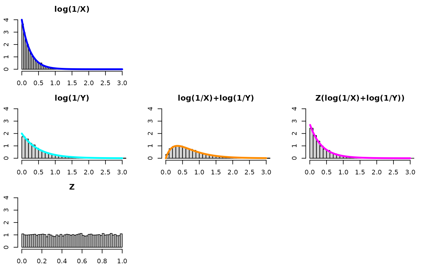
• $\left(X_1^{\alpha_1} X_2^{\alpha_2} \dots X_K^{\alpha_K} \right)^Z$ ~ Beta(1, 1)

Turns out there is another computed quantity with a distribution:

• $\left( \frac{1}{X_1^{\alpha_1} X_2^{\alpha_2} \dots X_K^{\alpha_K}} \right)^Z$ ~ Pareto(scale = 1, shape=1)

Let’s try it for summing 10 exponentials with different rates… and look at this new computed quantity.

This means we need Z to be “1/10 on average”. That is, we could draw 9 uniforms let Z be the minimum of those 9 uniforms. This is the same as letting Z ~ beta(1,10-1). The 10 is bolded, because this is the number of exponentials we’re summing, and it generalizes to any positive integer.

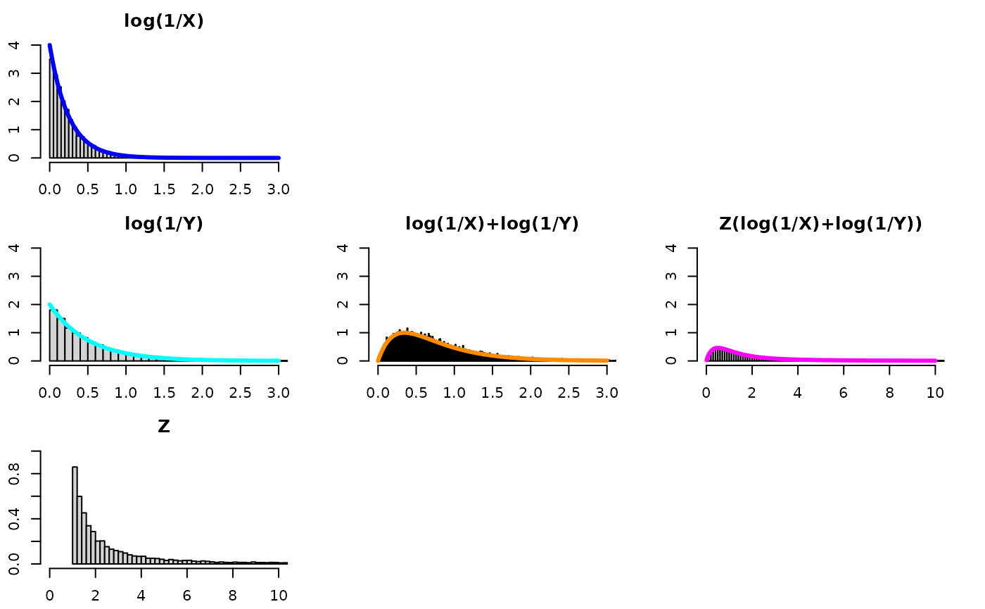
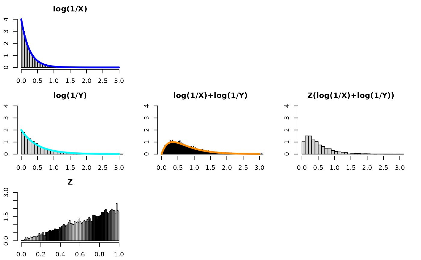
Be mindful of the x-axis and y-axis limits – they are not the same for every plot!

What if we did not change the computed quantity and kept it without any $\alpha$s as in part I? That’s the topic of the next session.

Way 2: Keep the Generalized Quantity – Investigate Z

In part I we considered cases where the alpha for X and Y are the same and how multiplying (log(1/X)+log(1/Y)) by Z allows one to recover the original distribution of log(1/X) (equivalently, log(1/Y)). However, if $\alpha_x \neq \alpha_y$, multiplying (log(1/X)+log(1/Y)) by a uniform would not recover the distribution for either log(1/X) or log(1/Y) – it would be a distribution “in-between” those two distributions – but not an Exponential with an alpha between $\alpha_x$ and $\alpha_y$. We consider this “unequal alpha” as a bonus case below.

What is the sum in the unequal rate case?

Firstly, one may want to consult Wikipedia.

• Wikipedia Sum of Two Independent Exponential Random Variables

So, in this setup, there is no one distribution to recover since $\alpha_x \neq \alpha_y$, so trying different distributions for $Z$ leads to different blends of the X,Y distributions for the quantity Z(log(1/X)+log(1/Y)).

Z distributed as U(0,1)

• $Z \sim$ U(0,1)
• magenta density
  • $f_w(w) = - \frac{mn \left( \Gamma(0,mw) - \Gamma(0,nw)\right)}{ m-n }$ where $W = Z \left( \log \frac{1}{X} + \log \frac{1}{Y} \right)$, m=$\alpha_x$, n=$\alpha_y$
  • $\Gamma(.,.)$ is incomplete Gamma function.

• While the computed quantity is not exponential, one can see it is a concentration of the convolution and that it is kind of “in-between” the two component distributions.

Z distributed as Inverse-Gamma(alpha, beta)

• $Z \sim$ Inverse-Gamma($\alpha_z$, $\beta_z$)

• gold density

  • $f_w(w) = \frac{mn}{ n-m }\frac{\beta_z^{\alpha_z}\Gamma(\alpha_z + 1)}{ \Gamma(\alpha_z) } \left( \frac{1}{ \left(mw+\beta_z\right)^{\alpha_z +1}}-\frac{1}{ \left(nw+\beta_z\right)^{\alpha_z +1}} \right)$ where $W = Z \left( \log \frac{1}{X} + \log \frac{1}{Y} \right)$, m=$\alpha_x$, n=$\alpha_y$.

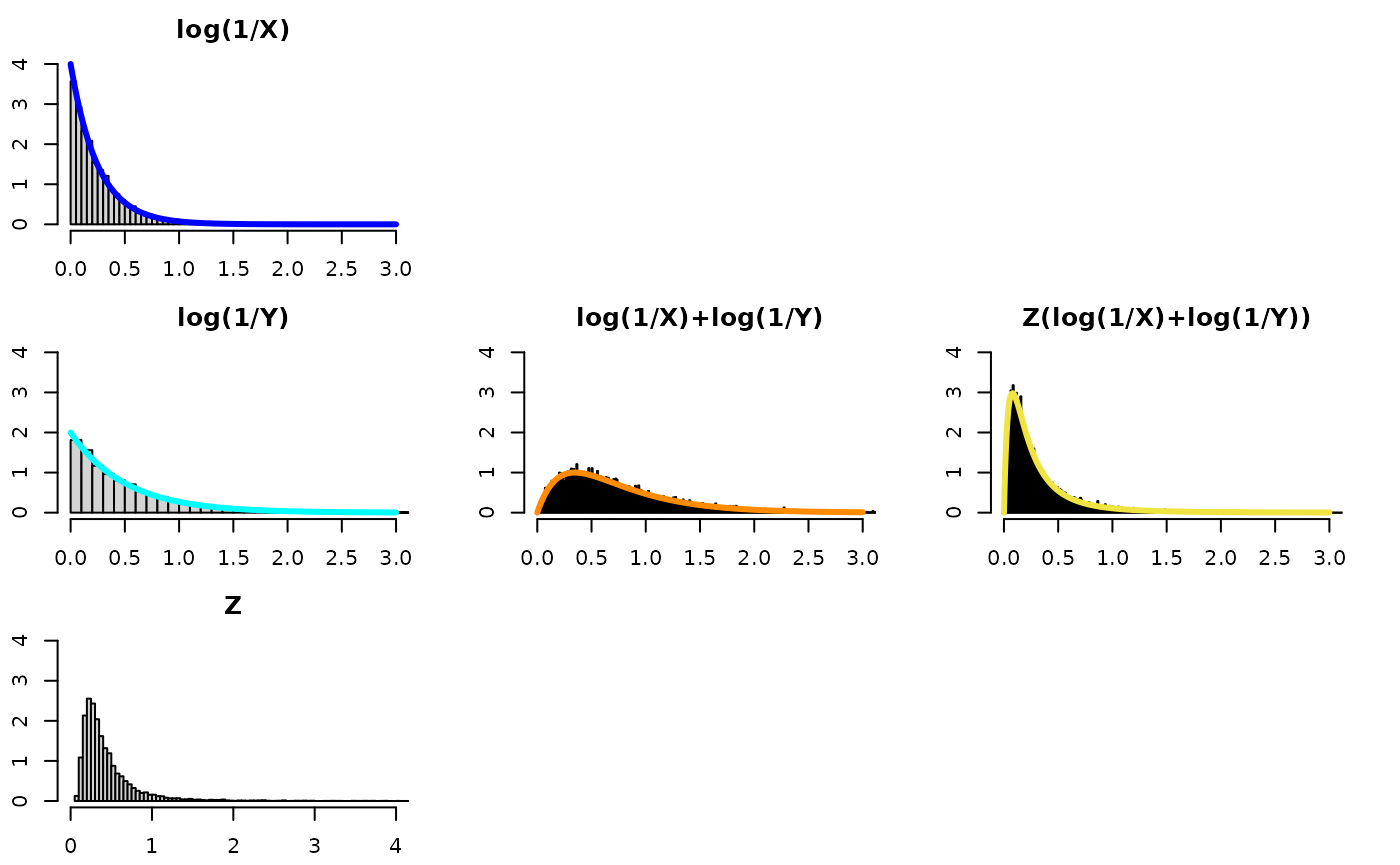
• While the computed quantity is not exponential, one can see it is a concentration of the convolution and that it is kind of “in-between” the two component distributions.

Z distributed as Pareto

• $Z \sim$ Pareto($x_m=1$,$\alpha_m=1$) (where 1/Z ~ U(0,1))

• magenta density:

  • $f_w(w) = \frac{n^2 (1-\exp^{-mw}(1+mw)) - m^2 (1-\exp^{-nw}(1+nw))}{ mn(n-m)w^2 }$ where $W = Z \left( \log \frac{1}{X} + \log \frac{1}{Y} \right)$, m=$\alpha_x$, n=$\alpha_y$.

• What is the opposite of “concentration” – bleeding out? Multiplying the convolution by a random number bigger than 1 disperses it.

Z distributed as ????